In this project, we will use different classification algorithms such as logistic regression, SVM, decision trees, and k-NN to predict whether a certain loan is paid off on time. We will then evaluate and compare their performance to select the best performing algorithm.

You can look at the Jupyter notebook here. In this project, I used the following Python libraries: Pandas, Matplotlib, Seaborn,and Scikit-learn. This project, in particular, required a significant amount of feature engineering.

The data includes details of 346 customers whose loan are already paid off or defaulted. Here is what it looks like:

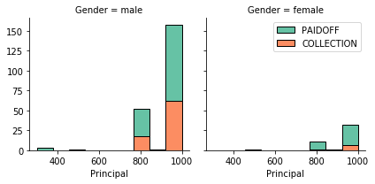
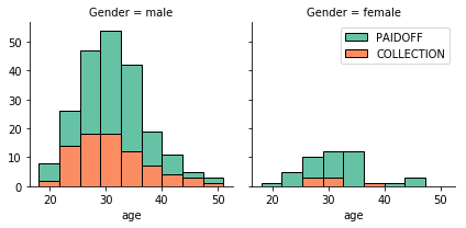
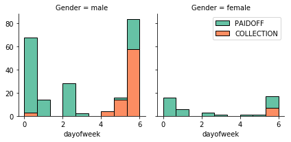
260 people have paid off the loan on time while 86 have gone into collection. In order to understand the breakdown of the data better, we can plot a couple of histograms.

After extracting the value for the day of the week from the ‘effective_date’ feature and plotting it in the histogram above, we see that people who get the loan at the end of the week are more likely to default on the loan so we can create a binary feature ‘weekend’ that tells us whether the loan began on a weekday or the weekend. Since gender is a binary categorical variable, we can simply code males as 0 and females as 1. As education has more than two levels, we can use one-hot encoding to create indicator variables for each feature.

The binary target variable ‘loan_status’ is imbalanced because more than 75% of the values are ‘PAIDOFF’. In such a situation, even a ‘simple’ model that predicts ‘PAIDOFF’ for every row would be able to attain 75% accuracy. As a consequence, we will not be using ‘accuracy’ (i.e. the percentage of correctly predicted labels) as a metric for model performance but will instead rely on the F1, Jaccard, and log-loss measures to judge model performance. These three measures are able to avoid the shortcomings of ‘accuracy’.

We will now use different classification algorithms such as k-NN, decision trees, SVM, and logistic regression to model our data. We will split the data into training and testing sets to ensure that the data used for training is not used for measuring model performance too.

For the k-Nearest Neighbors algorithm, we need to determine the optimal value of ‘k’ (the number of nearest neighbors) before we make our final model. We will achieve this through k-fold cross validation. In k-fold CV, the training set is split into k smaller sets. For each of the k “folds”, the following procedure is followed: A model is trained using k-1 of the folds as training data; the resulting model is validated on the remaining part of the data. The performance measure reported by k-fold cross-validation is then the average of the values computed in the loop. After implementing this procedure, we determine that k=7 is the optimal number.

Here we see the results of our models. We can see that SVM has performed better than all of the other models. One reason for k-NN’s relatively poor performance could be the fact that we used uniform weights for all of the neighbors. We could tinker with parameters like these to improve the model.

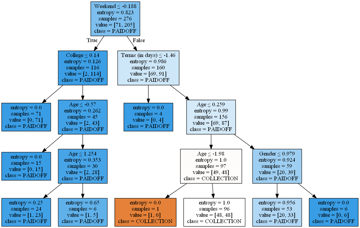
If we want somewhat of a balance between model complexity and model performance, decision trees could be a good option (Note: the decision tree below is based on normalized data).